Bayesian Inversion
Bayesian inference can be interpreted as a practical method for drawing conclusions of quantities from observed data using a statistical framework. The inherent probabilistic characteristic of the Bayesian approach allows a consistent quantification of uncertainties by a probability distribution. Therefore, it provides a better understanding of the risks supporting the decision that is based on the inference. Furthermore, the conclusions, as well as its uncertainties, can be easily updated as more evidence or information becomes available.
After setting the statistical model for the joint probability distribution for all the quantities of a problem, the inference of an unobserved quantity M is done by conditioning to the observed data D:
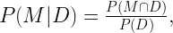
the fact that 

where 
Analogously, for continuous variables, the posterior distribution of a model parameter 


The Bayesian posterior distribution 


The relation between the observed data
Preferably, the prior distribution should be defined to contain information that are not covered by the likelihood, in order to solve the ambiguities that only with the observed data, the framework is not capable of. Nevertheless, the prior probabilities are intrinsically subjective and the choice of the distribution can drastically affect the posterior conclusions. Thus the prior definition is a challenge and should be carefully evaluated. For this reason, the difficulty in selecting a prior distribution is a fundamental drawback and it is the most criticized point of the Bayesian inference.
With the aim to reduce the prior influence on the resulting inference, several techniques were proposed, which gave more consistency and robustness for the Bayesian choice. The most popular techniques can be considered the conjugate, the hierarchical and the empirical prior modeling. Particularly, the conjugate prior modeling consists in the using of theoretical distribution as normal, Poisson, gamma and binomial, which allow an analytical treatment of the posterior distribution. Besides, more recently new developments have being presented, as sensitivity analysis, for the assessment of the influence of the prior. This process works as an efficient tool to evaluate the robustness of the prior distribution.
Another peculiarity of the Bayesian approach is the fact that the posterior distribution can be easily updated as more evidences and observed data become available. For example, the posterior distribution of the model parameter 


which can be extented to any number 


Bayesian approach for inverse problem
The goal of inverse modeling is to predict model variables from a parameterized physical system from observable data, theoretical relations between observable and unobservable parameters and prior information \cite{tarantola}. Usually, the model and the experimental data are represented by the vectors

where 
The forward model operator is, in general, a nonlinear operator based on theories or physical laws that allow the calculating of the experimental measurements, given a configuration of a parameterized physical system. Whereas the theory that allows the operator to simulate the observable data from the model, the inverse problem seeks just the opposite way, that is, to obtain the parameters of the model from the experimental data. More specifically, the seismic inversion seeks to obtain the rocks properties of the subsurface, through the artificial seismic acquisition and the theoretical relations of propagation of acoustic waves.
The most used techniques to solve inverse problems are the optimization methods as the Simulated Annealing, Genetic Algorithm, Ant Colony Optimization and Particle Swarm Optimization. However, very often there are noises, errors and ambiguities associated with the process that do not allow an accurate estimation of the model parameters. Another typical feature of the seismic inversion problems is the non-uniqueness of the solution, there are several models that satisfy the same given experimental seismic. Due to this reasons, the Bayesian inference is being present as the best choice to solve inverse problems, in which the posterior probability distribution over the parameters space is the most general solution and it allows a sound quantification of the uncertainties.