Monte Carlo Methods for Inverse Problems

25 Jul , 2017 sampling,statistics,white paper

The Monte Carlo method is a statistical method used in stochastic simulations with several applications in areas such as Physics, Mathematics and Biology. Its main feature is the use of random numbers in decision making. The name Monte Carlo is in reference to a casino that used a generator of random numbers in games of chance. One of the pioneers to use the method were Metropolis, 1953 and collaborators developing a simulation of a liquid in equilibrium with its gas phase. In order to obtain the thermal equilibrium of the system, they proposed that it would not be necessary to simulate the entire dynamics of the phenomenon, but only a Markov chain that follow the probability distribution function of the equilibrium.

In Statistical Physics the Metropolis Algorithm is used to study a wide variety of systems. A typical example is the application in the phase transitions studies, as the case of a fluid that reaches a limit temperature and solidifies. For the formation of a crystalline (solid) state without defects, a slow cooling needs to be done in the material. Otherwise, a metastable material is obtained, which corresponds to a defective crystal structure, outside of the minimal energy state. Finding the state of minimum energy, in Statistical mechanics, is an optimization problem with aspects common to combinatorial optimization.

The iterative procedures of global searching to solve optimization problems are similar to the processes in Statistical Mechanics. Small modifications applied to the parameter configuration with the aim of finding a better solution recall the rearrangements of microscopic configurations of the particles of a material, and the evaluation of the error function of the optimization problem can be described as an evaluation of the energy difference () between two microscopic states. This idea was explored by Kirkpatrick for the traveling salesman problem, which a certain parameter plays the role of temperature. But, unlike the Metropolis algorithm, the temperature (parameter) is not fixed and it decreases at each iteration. Such a method is known as Simulated Annealing.

There are several examples of the using of the Simulated Annealing and other optimization methods for seismic inversion. However, the unique solution that best matches an objective function, which is obtained by optimization techniques, does not consider any observation uncertainty and neither provides any information about the estimation uncertainties. Because of that, the using of the Monte Carlo methods for seismic inversion through Bayesian inference approach became popular during the last decades. Monte Carlo methods are used in seismic inversion due to the complexity of the posterior distribution, which can not usually be obtained analytically or sampled with traditional random number generation methods.

In the Bayesian approach, as discussed in the previous chapter, we wish to estimate the posterior probability distribution of the model parameters given the observed data and prior knowledge. In the cases that the posterior distribution can not be analytically derived, the distribution is computationally obtained by a Markov Chain, which in the stationary regime leads to configurations that follows the posterior distribution. Basically, a Markov Chain consists in a sequence of random variables with serial dependence only between adjacent components. For example, the Metropolis algorithm are able to perform a random walk, a sort of Brownian motion, where a new parameter configuration (obtained by a a random disturbance of the previous one) is accepted with a probability that depends on only the last parameter configuration . This acceptance factor is defined by the ratio of the posterior probabilities of each configuration:

which by the definition of the posterior probability distribution, can by written as:

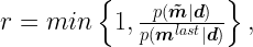
In practice, this acceptance factor makes the Metropolis algorithm to always accept new configurations that has a higher posterior probability (more suitable with the observed data and prior knowledge), although occasionally it also accepts bad configurations with lower posterior probability.

The algorithm starts with a given initial configuration and after some iterations, called burn-in period, the chain converges to the desired posterior distribution in the condition known as stationary regime. There is no general rule for how long the algorithm takes to reach this regime, it will strongly depend on the particular problem and how far the initial configuration is from the equilibrium values. Therefore, an initial number of samples are thrown away to properly compute the posterior distribution from the sampling.

In the particular cases that the prior probability density is simple and it can be sampled by traditional methods, the acceptance factor is calculated just using the ratio of the likelihoods of each configuration, because the prior sampling already generates configuration with probability . We can find applications with this approach for geophysical inverse problems, in which the prior distribution is a multivariate distribution with a given spatial correlation model, and it can be sampled by the geostatistical methods as Sequential Gaussian Simulation, Direct Sequential Simulation and FFT-Moving Average.

In the next subsections we discuss the Monte Carlo methods with more technical details. The Metropolis-Hastings algorithm is a generalization of the Metropolis one, which can be applied with asymmetric random steps. On the contrary, the Gibbs sampling is a special case of the Metropolis-Hastings, where all the new configurations are accepted.

Metropolis-Hastings algorithm

As the traditional Metropolis algorithm, the main idea of this method is simulating a random path as a Brownian motion, in which new configurations are obtained respecting some probabilistic rule, in order to converge to a desired distribution. More specifically, the sampling is performed by generating a Markov chain in the stationary regime, each new state of the chain corresponds to a sample of the desired distribution, for example the posterior probability density .

The algorithm consists in defining an initial configuration for the parameter of interest and then a new state is generated using the auxiliary distribution . The new configuration is accepted, or not, depending on the value of the acceptance factor  r given by

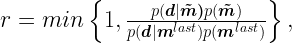
Notice that equation of the traditional Metropolis algorithm is a particular case of equation above when , which means that the probability of generate the configuration from is the same of generating from . Therefore, in applications where the parameters of the auxiliary distribution changes with respect to each iteration, or the way that the new configurations are generated, or even if is an asymmetric function, the traditional Metropolis equation must be used instead.

If the new configuration is accepted, on the other hand, if r <1, the new configuration is accepted with probability r. This procedure is repeated a number of times, depending on the number of samples we want to generate. An algorithm for the described method is presented below.

The variable k is the number of iterations required for the convergence of the chain to the stationary regime. In general, the chain is analyzed during the execution of the algorithm to identify the convergence. n is the number of samples that the algorithm will perform within the posterior distribution .

Gibbs sampling

A special case of the Metropolis algorithm was introduced by Geman and Geman, giving rise to the so-called Gibbs algorithm, or Gibbs sampling, which is an efficient way to obtain samples from the posterior distribution and the Bayesian inference.

The sampling algorithm is a particular case of the Metropolis algorithm, in which the auxialiary distribution is defined by the conditional distributions of each element of the model parameter, given all the other elements in a given iteration i:

where is the element and are all the others:

If we replace the Gibbs auxialiary distribution in  the traditional Metropolis equation, we have

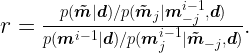
Reminding that and ,

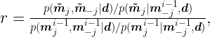
and by using the conditional probability rule, we conclude that

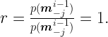
Thus, the method consists in executing, at each iteration  i, a sampling of all the elements of conditioned to the current state of the other elements. This technique ensures that the acceptance probability r of the Metropolis algorithm is always equal to 1. Therefore, the sampling by the Gibbs algorithm is faster, since it does not generate the non-existent states of the Markov chain. In this context, the Gibbs algorithm can be written as:

As discussed before, the Gibbs algorithm also needs a certain number of iterations k for the convergence to the stationary regime, and then it performs n samples within the desired distribution.

---